Tutorial: Using IPython/Jupyter Notebook with PyCharm
In this section:
- Before you start
- Creating a IPython Notebook file
- Filling in and running the first cell
- Working with cells
- Adding
- Clipboard operations with the cells
- Running and stopping kernels
- Choosing style
- Writing formulae
Before you start
Prior to executing the tasks of this tutorial, make sure that the following prerequisites are met:
- You have a Python project already created. In this tutorial the project
C:/SampleProjects/py/IPythonNotebookExampleis used. - In the Project Interpreter page of the
Settings/Preferences dialog, you have:
- Created a virtual environment. For this tutorial a virtual environment based on Python 3.5.0 has been created.
- Installed the following package:
jupyter
Note that PyCharm automatically installs the dependencies of these packages.
Creating a IPython Notebook file
In the Project tool window, click Alt+Insert. Then, on the pop-up
menu that appears, choose the option and type the file name (here it
is MatplotlibExample.ipynb).
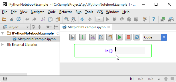
The newly created file now shows up in the Project tool window and automatically opens for editing.
By now, the new file is empty, but PyCharm recognizes it as a
notebook file.
As such, this file is marked with the icon ![]() and features a toolbar, which is a complete
replica of the real IPython Notebook toolbar:
and features a toolbar, which is a complete
replica of the real IPython Notebook toolbar:
Filling in and running the first cell
This is most easy. Just click the first cell and start typing. For example, in the very first cell type the
following code to configure the matplotlib package:
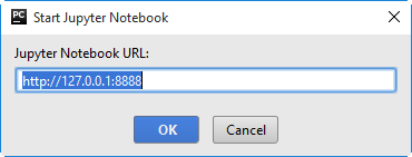
%matplotlib inlineNext, click the icon ![]() to run the cell (alternatively, you can press
Shift+Enter). PyCharm shows a dialog box, where you have to specify the URL where
the IPython Notebook server will run:
to run the cell (alternatively, you can press
Shift+Enter). PyCharm shows a dialog box, where you have to specify the URL where
the IPython Notebook server will run:
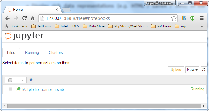
The console shows the server URL:
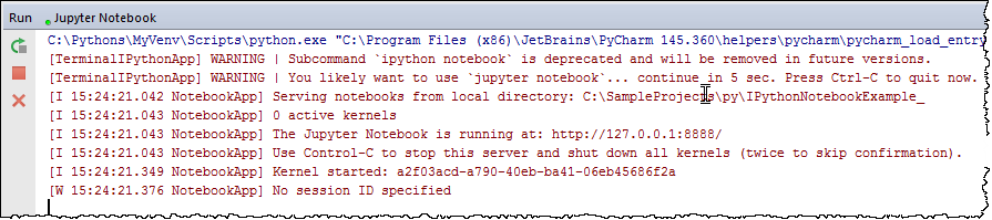
Follow this address:
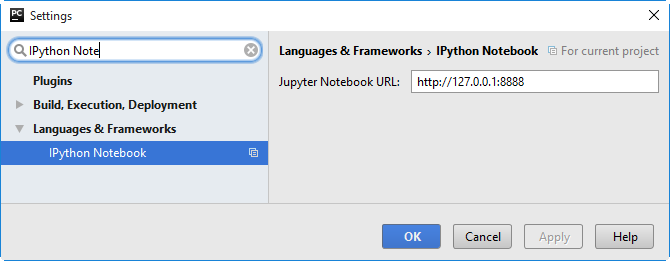
Note that the default URL is specified in the IPython Notebook page of the Settings/Preferences dialog:
Actually, that's it... From now on you are ready to work with the notebook integration.
Working with cells
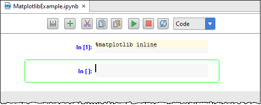
First of all, add the following import statement:
from pylab import *This how it's done. As you might have noticed, while you've run the first cell, PyCharm has automatically created the next empty cell:
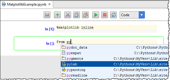
Start typing in this cell, and notice code completion:
Click ![]() on the toolbar again to run this cell. Note that the cell produces no output, but the
next empty cell is created automatically. In this new cell, enter the following code:
on the toolbar again to run this cell. Note that the cell produces no output, but the
next empty cell is created automatically. In this new cell, enter the following code:
figure()
plot(x, y, 'r')
xlabel('x')
ylabel('y')
title('title')
show()
Run this cell. Oops! The attempt to run results in an error:
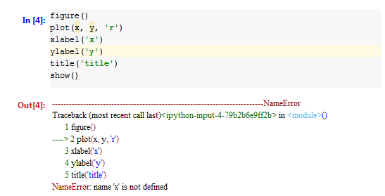
It seems that the variables should be defined first. To do that, add a new cell.
Adding
Since the new cell is added below the current one, click the cell with import statement - its frame
becomes green. Then on the toolbar click ![]() (or press Alt+Insert).
(or press Alt+Insert).
In the created cell, type the following code that will define x and
y variables:
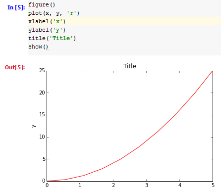
x = linspace(0, 5, 10)
y = x ** 2
Run this cell, and then run the next one. This time it shows the expected output:
Clipboard operations with the cells
Look at the toolbar. There are ![]() (Ctrl+C),
(Ctrl+C),
![]() (Ctrl+X), and
(Ctrl+X), and
![]() (Ctrl+V) buttons.
If you click
(Ctrl+V) buttons.
If you click ![]() , you thus delete the current cell, and take it into
the clipboard.
, you thus delete the current cell, and take it into
the clipboard.
Clicking ![]() results in inserting the contents of the clipboard
below the current cell. Finally,
results in inserting the contents of the clipboard
below the current cell. Finally, ![]() just duplicates the current cell.
just duplicates the current cell.
Try these buttons yourself.
Running and stopping kernels
As you've already learnt, the button ![]() is used to execute a cell.
is used to execute a cell.
If calculation of a certain cell takes too much time, you can always stop it. To do that, click ![]() on
the document toolbar.
on
the document toolbar.
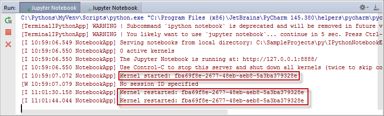
Finally, you can rerun the kernel by clicking ![]() on the document toolbar.
on the document toolbar.
The messages about all these actions show up in the console:
Choosing style
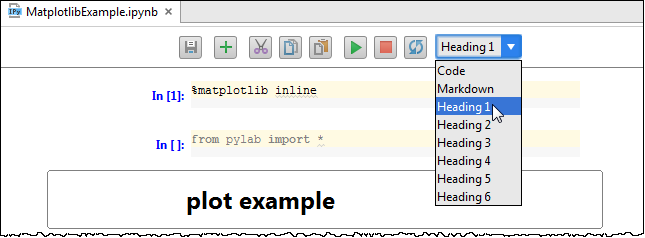
Look at the drop-down list to the right of the document toolbar. It allows you to choose presentation style of a cell. For example, the existing cells are presented as code.
Click the cell with the import statement again, and then click ![]() . The new cell appears
below. By default, its style selector shows
. The new cell appears
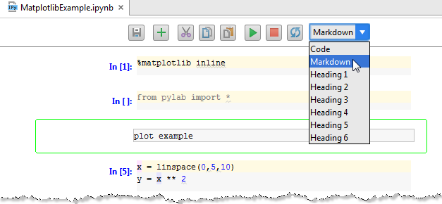
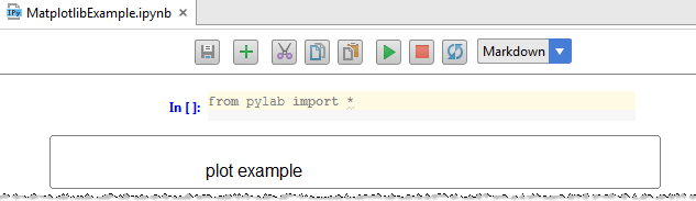
below. By default, its style selector shows Code. In this cell, type the
following text:
plot exampleNext, click the down arrow, and choose Markdown from the list. The cell changes its view:
Now click ![]() on the toolbar, and how the cell looks now:
on the toolbar, and how the cell looks now:
Now you can just select the desired style from the drop-down list, and the view of the cell changes appropriately:
Writing formulae
Add a new cell. In this cell, choose Markdown from the style selector, and type the following text:
$$c = \sqrt{a^2 + b^2}$$Click ![]() . The result is stunning:
. The result is stunning:
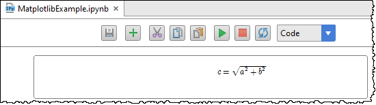
As you see, PyCharm's IPython Notebook integration makes it possible to use LaTex notation and render formulae, labels and text.
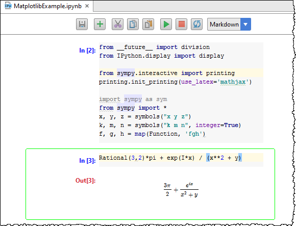
Next, explore the more complicated case. The expected result - the formula - should appear as the result of calculation. Add a cell and type the following code (taken from SymPy: Open Source Symbolic Mathematics):
from __future__ import division
from IPython.display import display

from sympy.interactive import printing
printing.init_printing(use_latex='mathjax')

import sympy as sym
from sympy import *
x, y, z = symbols("x y z")
k, m, n = symbols("k m n", integer=True)
f, g, h = map(Function, 'fgh')
Run this cell. It gives no output. Next, add another cell and type the following:
Rational(3,2)*pi + exp(I*x) / (x**2 + y)Click ![]() and enjoy:
and enjoy: